Understanding Big O Notation and Time Complexity

When developing algorithms, one of the most important considerations is their efficiency. We can measure efficiency in terms of time complexity, which indicates the amount of time an algorithm takes to run as a function of the size of its input. Big O notation is a mathematical representation used to describe the upper bound of an algorithm’s complexity. This blog will guide you through the concepts of Big O notation and how to calculate time complexity.

What is Big O Notation?

Big O notation provides a high-level understanding of the time or space complexity of an algorithm. It expresses the worst-case scenario of how an algorithm’s runtime or space requirements grow as the input size grows. The notation focuses on the dominant term and disregards lower-order terms and constant factors.

Common Big O Notation

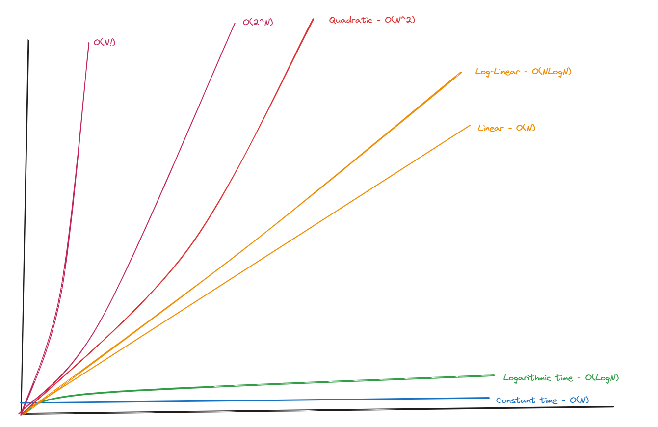
1. O(1): Constant time – The algorithm’s runtime is constant and does not depend on the input size.
2. O(log N): Logarithmic time – The runtime grows logarithmically with the input size.
3. O(N): Linear time – The runtime grows linearly with the input size.
4. O(N Log N): Linearithmic time – the runtime grows in proportion to N Log N.
5. O(N^2): Quadratic time – The runtime grows quadratically with the input size.
6. O(N!): Factorial time – The runtime grows factorially with the input size/

Calculating Time Complexity

To determine the time complexity of an algorithm, analyze the algorithm’s structure and the number of operations it performs relative to the input size.

Steps to Calculate Time Complexity

1. Identify the Basic Operations: Look for the fundamental operations that are being performed.
2. Count the Operations: Count how many times these operations are executed as a function of the input size.
3. Express in Big O Notation: Simplify the count to its Big O notation by focusing on the dominant term and ignoring constant factors and lower-order tems.

Example Analyses

Example 1: Constant Time – O(1)

def get_first_element(arr):
return arr[0]

• Analysis: This function performs a single operation regardless of the input size
• Time complexity: O(1)

Example 2: Linear Time – O(N)

def print_all_elements(arr):
    for element in arr:
        print(element)

• Analysis: This function performs loops through each element of the array once.
• Time complexity: O(N), where N is the length of the array.

Example 3: Quadratic Time – O(N^2)

def print_all_pairs(arr):
    for i in range(len(arr)):
        for j in range(len(arr)):
            print(arr[i], arr[j])

• Analysis: This function has a nested loop, each iteration N times.
• Time complexity: O(N^2), where N is the length of the array.

Example 4: Logarithmic Time – O(Log N)

def binary_search(arr, target):
    left, right = 0, len(arr) - 1
    while left <= right:
        mid = (left + right) // 2
        if arr[mid] == target:
            return mid
        elif arr[mid] < target:
            left = mid + 1
        else:
            right = mid - 1
    return -1

• Analysis: This function halves the search space each iteration.
• Time Complexity: O(Log N)

Simplifying Time Complexity

When expressing time complexity in Big O notation, focus on the term that grows the fastest as the input size increases, and drop constant factors and lower-order teams. Here are some examples:

• O(2N + 3) simplifies to O(N)
• O(N + N^2) simplifies to O(N^2)
• O(3N LogN + 100) simplifies to O(N Log N).

Practice Tips

1. Ignore Constants: Big O notation disregards constants and smaller terms because they become insignificant for large inputs.
2. Consider Worst Case: Focus on the worst-case scenario for a comprehensive analysis.
3. Use Dominant Terms: Identify the tern that grows the fastest and use it to represent the time complexity.

Common Algorithm Time Complexities

• Accessing an element in an array: O(1)
• Searching for an element in a sorted array (Binary Search): O(log N)
• Inserting an element in a sorted array: O(N)
• Merging two sorted arrays: O(N)
• Quicksort: O(N log N) on average, O(N^2) in the worst case
• Heapsort: O(N log N)
• Matrix multiplication: O(N^3)

Conclusion

Understanding Big O notation and how to calculate time complexity is crucial for designing efficient algorithms. By analyzing an algorithm’s time complexity, you can make informed decisions about the best approach for solving a problem, especially as the input size grows. Mastering these concepts will enhance your ability to write optimized and scalable code.